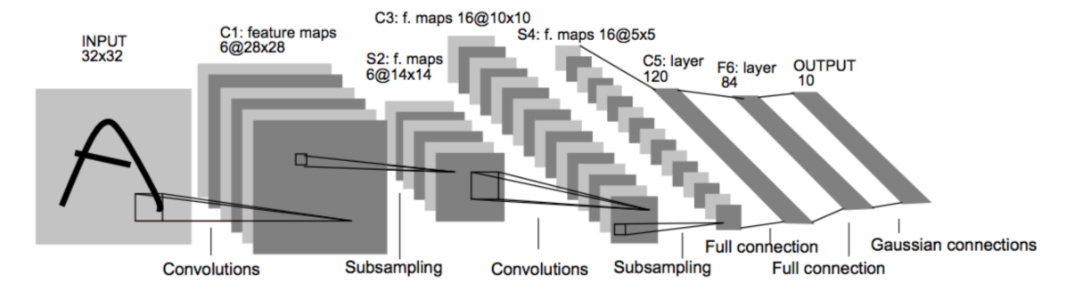
LeNet由Yann Lecun 提出,是一种经典的卷积神经网络,是现代卷积神经网络的起源之一。Yann将该网络用于邮局的邮政的邮政编码识别,有着良好的学习和识别能力。LeNet又称LeNet-5,具有一个输入层,两个卷积层,两个池化层,3个全连接层(其中最后一个全连接层为输出层)。
1.MLP
多层感知机MLP(Multilayer Perceptron),也是人工神经网络(ANN,Artificial Neural Network),是一种全连接(全连接:MLP由多个神经元按照层次结构组成,每个神经元都与上一层的所有神经元相连)的前馈神经网络模型。
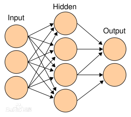
多层感知机(Multilayer Perceptron, MLP)是一种前馈神经网络,它由输入层、若干隐藏层和输出层组成。每一层都由多个神经元(或称为节点)组成。
- 输入层(Input Layer):输入层接收外部输入的数据,将其传递到下一层。每个输入特征都对应一个神经元。
- 隐藏层(Hidden Layer):隐藏层是位于输入层和输出层之间的一层或多层神经元。每个隐藏层的神经元接收上一层传来的输入,并通过权重和激活函数进行计算,然后将结果传递到下一层。隐藏层的存在可以使多层感知机具备更强的非线性拟合能力。
- 输出层(Output Layer):输出层接收隐藏层的输出,并产生最终的输出结果。输出层的神经元数目通常与任务的输出类别数目一致。对于分类任务,输出层通常使用softmax激活函数来计算每个类别的概率分布;对于回归任务,输出层可以使用线性激活函数。
多层感知机的各层之间是全连接的,也就是说,每个神经元都与上一层的每个神经元相连。每个连接都有一个与之相关的权重和一个偏置。
2.LeNet简介
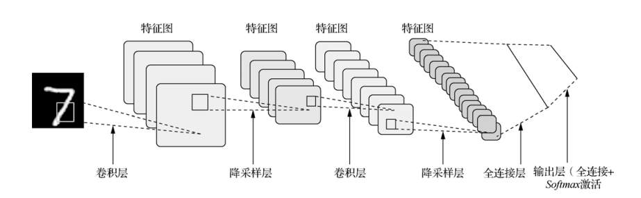
LeNet-5模型是由杨立昆(Yann LeCun)教授于1998年在论文Gradient-Based Learning Applied to Document Recognition中提出的,是一种用于手写体字符识别的非常高效的卷积神经网络,其实现过程如下图所示。
原论文的经典的LeNet-5网络结构如下:
各个结构作用:
卷积层:提取特征图的特征,浅层的卷积提取的是一些纹路、轮廓等浅层的空间特征,对于深层的卷积,可以提取出深层次的空间特征。
池化层: 1、降低维度 2、最大池化或者平均池化,在本网络结构中使用的是最大池化。
全连接层: 1、输出结果 2、位置:一般位于CNN网络的末端。 3、操作:需要将特征图reshape成一维向量,再送入全连接层中进行分类或者回归。
下来我们使用代码详解推理一下各卷积层参数的变化:
import torch
import torch.nn as nn

# 定义张量x,它的尺寸是1×1×28×28
# 表示了1个,单通道,32×32大小的数据
x = torch.zeros([1, 1, 32, 32])
# 定义一个输入通道是1,输出通道是6,卷积核大小是5x5的卷积层
conv1 = nn.Conv2d(in_channels=1, out_channels=6, kernel_size=5)
# 将x,输入至conv,计算出结果c
c1 = conv1(x)
# 打印结果尺寸程序输出:
print(c1.shape)

# 定义最大池化层
pool = nn.MaxPool2d(2)
# 将卷积层计算得到的特征图c,输入至pool
s1 = pool(c1)
# 输出s的尺寸
print(s1.shape)

# 定义第二个输入通道是6,输出通道是16,卷积核大小是5x5的卷积层
conv2 = nn.Conv2d(in_channels=6, out_channels=16, kernel_size=5)
# 将x,输入至conv,计算出结果c
c2 = conv2(s1)
# 打印结果尺寸程序输出:
print(c2.shape)

s2 = pool(c2)
# 输出s的尺寸
print(s2.shape)
输出结果:
torch.Size([1, 6, 28, 28])
torch.Size([1, 6, 14, 14])
torch.Size([1, 16, 10, 10])
torch.Size([1, 16, 5, 5])
下面是使用pytorch实现一个最简单的LeNet模型。
import torch
import torch.nn as nn
import torch.nn.functional as F


class LeNet(nn.Module):
    def __init__(self):
        super(LeNet, self).__init__()
        # 定义卷积层
        self.conv1 = nn.Conv2d(in_channels=1, out_channels=6, kernel_size=5, stride=1)
        self.conv2 = nn.Conv2d(in_channels=6, out_channels=16, kernel_size=5, stride=1)

        # 定义全连接层
        self.fc1 = nn.Linear(16 * 5 * 5, 120)
        self.fc2 = nn.Linear(120, 84)
        self.fc3 = nn.Linear(84, 10)

        # 定义激活函数
        self.relu = nn.ReLU()

    def forward(self, x):
        # 卷积层 + 池化层 + 激活函数
        x = self.relu(self.conv1(x))
        x = F.avg_pool2d(x, kernel_size=2, stride=2)
        x = self.relu(self.conv2(x))
        x = F.avg_pool2d(x, kernel_size=2, stride=2)

        # 展平特征图
        x = torch.flatten(x, 1)

        # 全连接层
        x = self.relu(self.fc1(x))
        x = self.relu(self.fc2(x))
        x = self.fc3(x)

        return x

# 创建模型实例
model = LeNet()

# 打印模型结构
print(model)
输出结果:
LeNet(
  (conv1): Conv2d(1, 6, kernel_size=(5, 5), stride=(1, 1))
  (conv2): Conv2d(6, 16, kernel_size=(5, 5), stride=(1, 1))
  (fc1): Linear(in_features=400, out_features=120, bias=True)
  (fc2): Linear(in_features=120, out_features=84, bias=True)
  (fc3): Linear(in_features=84, out_features=10, bias=True)
  (relu): ReLU()
)
3.Mnist数据集
MNIST是一个手写数字集合,该数据集来自美国国家标准与技术研究所, National Institute of Standards and Technology (NIST). 训练集 (training set) 由来自 250 个不同人手写的数字构成, 其中 50% 是高中学生, 50% 来自人口普查局 (the Census Bureau) 的工作人员. 测试集(test set) 也是同样比例的手写数字数据。
3.1 MNIST数据集简介
- 该数据集包含60,000个用于训练的示例和10,000个用于测试的示例。
- 数据集包含了0-9共10类手写数字图片,每张图片都做了尺寸归一化,都是28x28大小的灰度图。
- MNIST数据集包含四个部分: 训练集图像:train-images-idx3-ubyte.gz(9.9MB,包含60000个样本) 训练集标签:train-labels-idx1-ubyte.gz(29KB,包含60000个标签) 测试集图像:t10k-images-idx3-ubyte.gz(1.6MB,包含10000个样本) 测试集标签:t10k-labels-idx1-ubyte.gz(5KB,包含10000个标签)
3.2 MNIST数据集的预处理
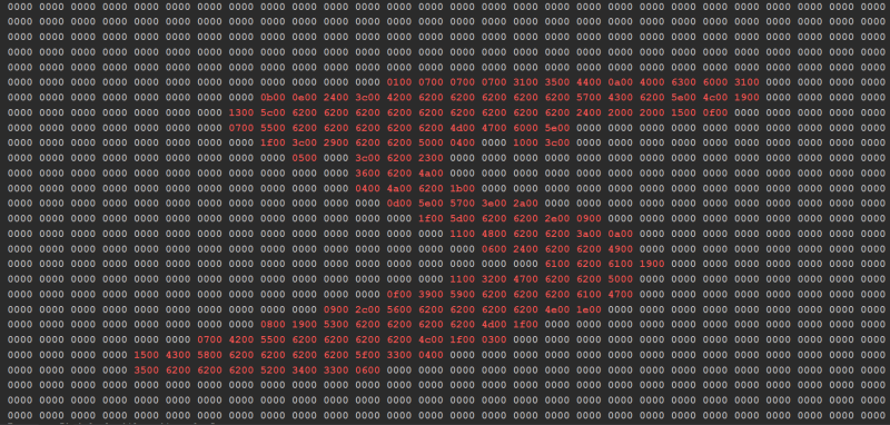
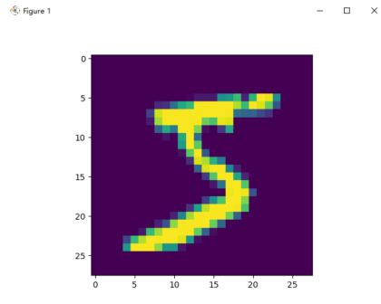
这里我们可以观察训练集、验证集、测试集分别有50000,10000,10000张图片,并且读取训练集的第一张图片看看。
import matplotlib.pyplot as plt
import numpy as np
import _pickle as cPickle
import gzip
import struct


def vectorized_result(j):
    e = np.zeros((10, 1))
    e[j] = 1.0
    return e


f = gzip.open("./data/mnist/mnist.pkl.gz", 'rb')
training_data, validation_data, test_data = cPickle.load(f, encoding='bytes')

print(len(training_data[0]))
print(len(validation_data[0]))
print(len(test_data[0]))

print(len(training_data))  # 包含图像和标签两个维度
print(training_data[0][0].shape)  # 50000张784*1的图像
print(training_data[1].shape)  # 50000个数字标签

print("=" * 140)

data = training_data[0][0]  # 一维列表
rows = 28  # 行数
columns = 28  # 列数

# 重新组织为二维矩阵
matrix = [data[i * columns: (i + 1) * columns] for i in range(rows)]
counter = 0
# 输出矩阵
for row in matrix:
    for value in row:
        # 方法1:取整数部分
        integer_part = int(value * 100)

        # 将整数转换为2个字节的十六进制表示
        hex_bytes = struct.pack('H', integer_part)
        hex_string = hex_bytes.hex()  # 转换为十六进制字符串
        if hex_string == '0000':
            print(hex_string + ' ', end="")
        else:
            print(f'\033[31m{hex_string}\033[0m' + " ", end="")
        counter += 1
        if counter % 28 == 0:
            print("", end='\n')
    # print(' '.join(map(str, b)))

print("=" * 140)
training_inputs = [np.reshape(x, (784, 1)) for x in training_data[0]]
training_results = [vectorized_result(y) for y in training_data[1]]
training_data = list(zip(training_inputs, training_results))

validation_inputs = [np.reshape(x, (784, 1)) for x in validation_data[0]]
validation_data = list(zip(validation_inputs, validation_data[1]))

test_inputs = [np.reshape(x, (784, 1)) for x in test_data[0]]
test_data = list(zip(test_inputs, test_data[1]))

img = training_inputs[0]
img = img.reshape(28, -1)
print(type(img))
plt.imshow(img)
plt.show()
输出结果:
50000
10000
10000
2
(784,)
(50000,)
4.LeNet手写数字识别
代码实现如下:
import torch
import torch.nn as nn
import torch.nn.functional as F
import torch.optim as optim
from torchvision import datasets, transforms
import time
from matplotlib import pyplot as plt
pipline_train = transforms.Compose([
# 随机旋转图片
transforms.RandomHorizontalFlip(),
# 将图片尺寸resize到32x32
transforms.Resize((32, 32)),
# 将图片转化为Tensor格式
transforms.ToTensor(),
# 正则化(当模型出现过拟合的情况时,用来降低模型的复杂度)
transforms.Normalize((0.1307,), (0.3081,))
])
pipline_test = transforms.Compose([
# 将图片尺寸resize到32x32
transforms.Resize((32, 32)),
transforms.ToTensor(),
transforms.Normalize((0.1307,), (0.3081,))
])
# 下载数据集
train_set = datasets.MNIST(root="./dataset", train=True, download=True, transform=pipline_train)
test_set = datasets.MNIST(root="./dataset", train=False, download=True, transform=pipline_test)
# 加载数据集
trainloader = torch.utils.data.DataLoader(train_set, batch_size=64, shuffle=True)
testloader = torch.utils.data.DataLoader(test_set, batch_size=32, shuffle=False)
#构建LeNet模型
class LeNet(nn.Module):
def __init__(self):
super(LeNet, self).__init__()
self.conv1 = nn.Conv2d(1, 6, 5)
self.relu = nn.ReLU()
self.maxpool1 = nn.MaxPool2d(2, 2)
self.conv2 = nn.Conv2d(6, 16, 5)
self.maxpool2 = nn.MaxPool2d(2, 2)
self.fc1 = nn.Linear(16 * 5 * 5, 120)
self.fc2 = nn.Linear(120, 84)
self.fc3 = nn.Linear(84, 10)
def forward(self, x):
x = self.conv1(x)
x = self.relu(x)
x = self.maxpool1(x)
x = self.conv2(x)
x = self.maxpool2(x)
x = x.view(-1, 16 * 5 * 5)
x = F.relu(self.fc1(x))
x = F.relu(self.fc2(x))
x = self.fc3(x)
output = F.log_softmax(x, dim=1)
return output
# 创建模型,部署gpu
device = torch.device("cuda" if torch.cuda.is_available() else "cpu")
model = LeNet().to(device)
# 定义优化器
optimizer = optim.Adam(model.parameters(), lr=0.001)
def train_runner(model, device, trainloader, optimizer, epoch):
# 训练模型, 启用 BatchNormalization 和 Dropout, 将BatchNormalization和Dropout置为True
model.train()
total = 0
correct = 0.0
# enumerate迭代已加载的数据集,同时获取数据和数据下标
for i, data in enumerate(trainloader, 0):
inputs, labels = data
# 把模型部署到device上
inputs, labels = inputs.to(device), labels.to(device)
# 初始化梯度
optimizer.zero_grad()
# 保存训练结果
outputs = model(inputs)
# 计算损失和
# 多分类情况通常使用cross_entropy(交叉熵损失函数), 而对于二分类问题, 通常使用sigmod
loss = F.cross_entropy(outputs, labels)
# 获取最大概率的预测结果
# dim=1表示返回每一行的最大值对应的列下标
predict = outputs.argmax(dim=1)
total += labels.size(0)
correct += (predict == labels).sum().item()
# 反向传播
loss.backward()
# 更新参数
optimizer.step()
if i % 1000 == 0:
# loss.item()表示当前loss的数值
print(
"Train Epoch{} \t Loss: {:.6f}, accuracy: {:.6f}%".format(epoch, loss.item(), 100 * (correct / total)))
Loss.append(loss.item())
Accuracy.append(correct / total)
return loss.item(), correct / total
def test_runner(model, device, testloader):
# 模型验证, 必须要写, 否则只要有输入数据, 即使不训练, 它也会改变权值
# 因为调用eval()将不启用 BatchNormalization 和 Dropout, BatchNormalization和Dropout置为False
model.eval()
# 统计模型正确率, 设置初始值
correct = 0.0
test_loss = 0.0
total = 0
# torch.no_grad将不会计算梯度, 也不会进行反向传播
with torch.no_grad():
for data, label in testloader:
data, label = data.to(device), label.to(device)
output = model(data)
test_loss += F.cross_entropy(output, label).item()
predict = output.argmax(dim=1)
# 计算正确数量
total += label.size(0)
correct += (predict == label).sum().item()
# 计算损失值
print("test_avarage_loss: {:.6f}, accuracy: {:.6f}%".format(test_loss / total, 100 * (correct / total)))
# 调用
epoch = 5
Loss = []
Accuracy = []
for epoch in range(1, epoch + 1):
print("start_time", time.strftime('%Y-%m-%d %H:%M:%S', time.localtime(time.time())))
loss, acc = train_runner(model, device, trainloader, optimizer, epoch)
Loss.append(loss)
Accuracy.append(acc)
test_runner(model, device, testloader)
print("end_time: ", time.strftime('%Y-%m-%d %H:%M:%S', time.localtime(time.time())), '\n')
print('Finished Training')
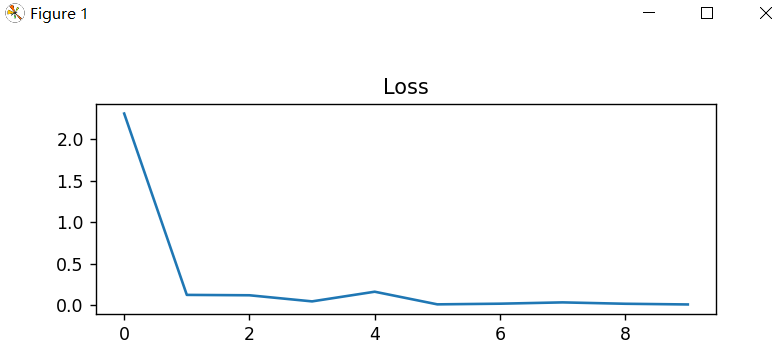
plt.subplot(2, 1, 1)
plt.plot(Loss)
plt.title('Loss')
plt.show()
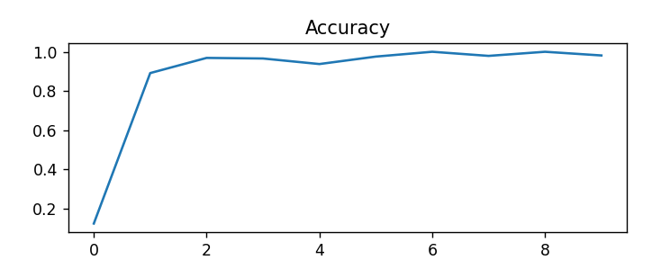
plt.subplot(2, 1, 2)
plt.plot(Accuracy)
plt.title('Accuracy')
plt.show()
输出效果:
start_time 2025-03-04 22:58:02
Train Epoch1     Loss: 2.310468, accuracy: 12.500000%
test_avarage_loss: 0.003581, accuracy: 96.450000%
end_time:  2025-03-04 22:58:24

start_time 2025-03-04 22:58:24
Train Epoch2     Loss: 0.121443, accuracy: 96.875000%
test_avarage_loss: 0.002549, accuracy: 97.220000%
end_time:  2025-03-04 22:58:47

start_time 2025-03-04 22:58:47
Train Epoch3     Loss: 0.164226, accuracy: 93.750000%
test_avarage_loss: 0.001965, accuracy: 98.000000%
end_time:  2025-03-04 22:59:10

start_time 2025-03-04 22:59:10
Train Epoch4     Loss: 0.019988, accuracy: 100.000000%
test_avarage_loss: 0.002175, accuracy: 97.820000%
end_time:  2025-03-04 22:59:33

start_time 2025-03-04 22:59:33
Train Epoch5     Loss: 0.019168, accuracy: 100.000000%
test_avarage_loss: 0.001945, accuracy: 98.000000%
end_time:  2025-03-04 22:59:56

Finished Training
增加模型预测功能。
model.load_state_dict(torch.load('./mymodel.pt'))
print("成功加载模型....")

index = random.randint(0,100)
image, label = train_set[index]  # 从 test_set 中直接获取图像和标签
image = image.unsqueeze(0).to(device)

# 进行预测
model.eval()
with torch.no_grad():
    output = model(image)
    predicted_label = output.argmax(dim=1, keepdim=True)

print("Predicted label:", predicted_label[0].item())
print("Actual label:", label)
运行效果:
成功加载模型....

Predicted label: 9
Actual label: 9