1.情感分析

情感分析就像是给文字装上了一个“情绪探测器”，它能告诉机器一段文字是开心的、生气的、难过的，还是中立的。简单来说，就是让机器读懂人类的情绪。

想象一下，你在看一条评论： - “这部电影太棒了！演员演得太好了！” → 这是正面情绪（开心、喜欢）。 - “这部电影真糟糕！浪费时间！” → 这是负面情绪（生气、讨厌）。 - “这部电影还行吧，没什么特别的。” → 这是中立情绪（没情绪，或者情绪不明显）。

情感分析就是让机器自动判断这些文字的情绪，就像一个“情绪机器人”在帮你分析。

Scapy实现情感分析：

import spacy
from textblob import TextBlob

# 加载Spacy的英语模型
nlp = spacy.load("en_core_web_trf")

# 示例文本
text = "I love this library. It is amazing and helpful!"

# 使用Spacy进行文本处理
doc = nlp(text)

# 使用TextBlob进行情感分析
for sentence in doc.sents:
    blob = TextBlob(sentence.text)
    print(f"句子: {sentence.text}, 情感分析: {blob.sentiment}")

运行效果：

句子: I love this library., 情感分析: Sentiment(polarity=0.5, subjectivity=0.6)
句子: It is amazing and helpful!, 情感分析: Sentiment(polarity=0.7500000000000001, subjectivity=0.9)

NLTK实现情感分析：

# 导入必要的库
import nltk
import jieba
from collections import defaultdict

# 下载NLTK数据包
nltk.download('punkt')

# 准备中文情感词典
positive_words = set(['好', '喜欢', '爱', '满意', '开心'])
negative_words = set(['差', '讨厌', '恨', '不满意', '伤心'])

# 准备中文停用词列表
stop_words = set(['的', '了', '和', '是', '在', '我', '你', '他'])

# 分词函数
def tokenize_text(text):
    return jieba.lcut(text)

# 去除停用词函数
def remove_stopwords(tokens, stop_words):
    return [token for token in tokens if token not in stop_words]

# 情感分析函数
def analyze_sentiment(text, positive_words, negative_words, stop_words):
    # 分词
    tokens = tokenize_text(text)
    # 去除停用词
    filtered_tokens = remove_stopwords(tokens, stop_words)
    # 计算情感得分
    score = 0
    for token in filtered_tokens:
        if token in positive_words:
            score += 1
        elif token in negative_words:
            score -= 1
    # 判断情感倾向
    if score > 0:
        return 'Positive'
    elif score < 0:
        return 'Negative'
    else:
        return 'Neutral'

# 示例文本
text = "这个产品真的很好，我很喜欢！"

# 进行情感分析
sentiment = analyze_sentiment(text, positive_words, negative_words, stop_words)
print(f"文本: {text}")
print(f"情感分析结果: {sentiment}")

运行效果：

文本: 这个产品真的很好，我很喜欢！
情感分析结果: Positive

2.NLP文本情感分析案例

人们对产品、服务、组织、个人、问题、事件、话题及其属性的观点、情 感、情绪、评价和态度的计算研究。文本情感分析（Sentiment Analysis）是自然语言处理（NLP）方法中常见的应用，也是一个有趣的基本任务，尤其是以提炼文本情绪内容为目的的分类。它是对带有情感色彩的主观性文本进行分析、处理、归纳和推理的过程。

本文将介绍情感分析中的情感极性（倾向）分析。所谓情感极性分析，指的是对文本进行褒义、贬义、中性的判断。在大多应用场景下，只分为两类。例如对于“喜爱”和“厌恶”这两个词，就属于不同的情感倾向。

下来将详细介绍如何进行文本数据预处理，并使用深度学习模型中的LSTM模型来实现文本的情感分析。

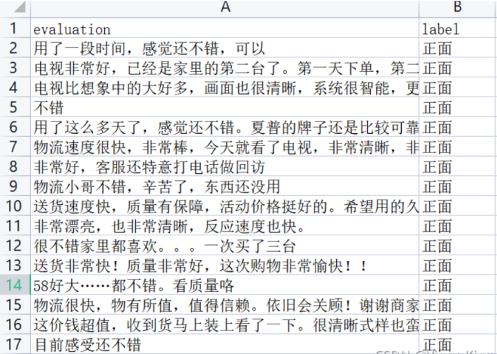
我们以某电商网站中某个商品的评论作为语料（corpus.csv），点击下载数据集，该数据集一共有4310条评论数据，文本的情感分为两类：“正面”和“反面”，该数据集的前几行如下：

1）.数据集分析

• 数据集中的情感分布
• 数据集中的评论句子长度分布

以下代码为统计数据集中的情感分布以及评论句子长度分布。

首先安装pandas和matplotlib依赖。

pip install pandas
pip install matplotlib

import pandas as pd
import matplotlib.pyplot as plt
from matplotlib import font_manager
from itertools import accumulate

# 设置matplotlib绘图时的字体
my_font = font_manager.FontProperties(fname="C:\Windows\Fonts\simhei.ttf")

# 统计句子长度及长度出现的频数
df = pd.read_csv('data/data_single.csv')
print(df.groupby('label')['label'].count())

df['length'] = df['evaluation'].apply(lambda x: len(x))
len_df = df.groupby('length').count()
sent_length = len_df.index.tolist()
sent_freq = len_df['evaluation'].tolist()

# 绘制句子长度及出现频数统计图
plt.bar(sent_length, sent_freq)
plt.title('句子长度及出现频数统计图', fontproperties=my_font)
plt.xlabel('句子长度', fontproperties=my_font)
plt.ylabel('句子长度出现的频数', fontproperties=my_font)
plt.show()
plt.close()
# 绘制句子长度累积分布函数(CDF)
sent_pentage_list = [(count / sum(sent_freq)) for count in accumulate(sent_freq)]

# 绘制CDF
plt.plot(sent_length, sent_pentage_list)

# 寻找分位点为quantile的句子长度
quantile = 0.91
print(list(sent_pentage_list))
for length, per in zip(sent_length, sent_pentage_list):
    if round(per, 2) == quantile:
        index = length
        break
print('\n分位点维%s的句子长度：%d.' % (quantile, index))

plt.show()
plt.close()

# 绘制句子长度累积分布函数图
plt.plot(sent_length, sent_pentage_list)
plt.hlines(quantile, 0, index, colors='c', linestyles='dashed')
plt.vlines(index, 0, quantile, colors='c', linestyles='dashed')
plt.text(0, quantile, str(quantile))
plt.text(index, 0, str(index))
plt.title('句子长度累计分布函数图', fontproperties=my_font)
plt.xlabel('句子长度', fontproperties=my_font)
plt.ylabel('句子长度累积频率', fontproperties=my_font)
plt.show()
plt.close()

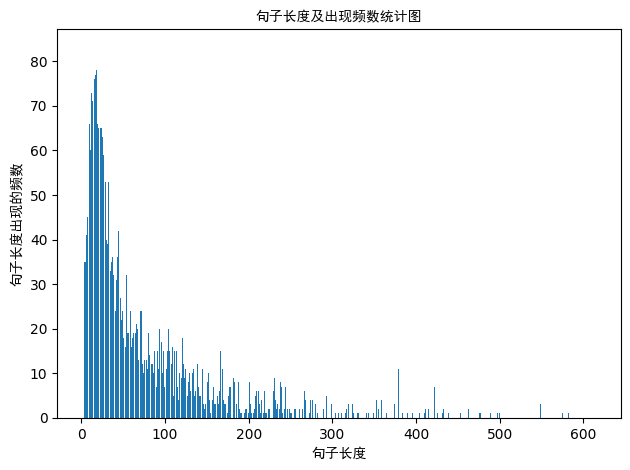
句子长度及出现频数统计图如下：

句子长度累积分布函数图如下：

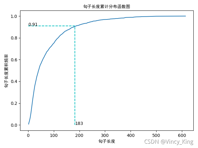
从以上的图片可以看出，大多数样本的句子长度集中在1-200之间，句子长度累计频率取0.91分位点，则长度为183左右。

2).LSTM模型

实现的模型框架如下：

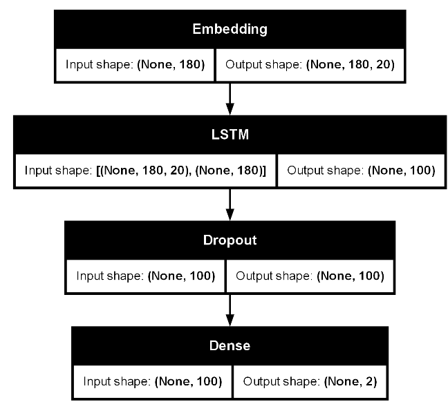
实现代码如下：

首先安装以下依赖。

pip install tensorflow
pip install scikit-learn
pip install graphviz
pip install pydot

注意：我们必须先下载安装graphviz。graphviz (英文：Graph Visualization Software的缩写）是一个由AT&T实验室启动的开源工具包，用于绘制DOT语言脚本描述的图形。

graphviz 下载地址如下：

https://graphviz.org/download/

Tensorflow实现：

import pickle

import keras
import numpy as np
import pandas as pd
import tensorflow as tf
from keras.src.utils import plot_model, pad_sequences
from keras.src.models import Sequential
from keras.src.layers import LSTM, Dense, Embedding,Dropout
from sklearn.model_selection import train_test_split
from sklearn.metrics import accuracy_score

# load dataset
# ['evaluation'] is feature, ['label'] is label
def load_data(filepath,input_shape=20):
    df=pd.read_csv(filepath)

    # 标签及词汇表
    labels,vocabulary=list(df['label'].unique()),list(df['evaluation'].unique())

    # 构造字符级别的特征
    string=''
    for word in vocabulary:
        string+=word

    vocabulary=set(string)

    # 字典列表
    word_dictionary={word:i+1 for i,word in enumerate(vocabulary)}
    with open('word_dict.pk','wb') as f:
        pickle.dump(word_dictionary,f)
    inverse_word_dictionary={i+1:word for i,word in enumerate(vocabulary)}
    label_dictionary={label:i for i,label in enumerate(labels)}
    with open('label_dict.pk','wb') as f:
        pickle.dump(label_dictionary,f)
    output_dictionary={i:labels for i,labels in enumerate(labels)}

    # 词汇表大小
    vocab_size=len(word_dictionary.keys())
    # 标签类别数量
    label_size=len(label_dictionary.keys())

    # 序列填充，按input_shape填充，长度不足的按0补充
    x=[[word_dictionary[word] for word in sent] for sent in df['evaluation']]
    x=pad_sequences(maxlen=input_shape,sequences=x,padding='post',value=0)
    y=[[label_dictionary[sent]] for sent in df['label']]
    '''
    np_utils.to_categorical用于将标签转化为形如(nb_samples, nb_classes)
    的二值序列。
    假设num_classes = 10。
    如将[1, 2, 3,……4]转化成：
    [[0, 1, 0, 0, 0, 0, 0, 0]
     [0, 0, 1, 0, 0, 0, 0, 0]
     [0, 0, 0, 1, 0, 0, 0, 0]
    ……
    [0, 0, 0, 0, 1, 0, 0, 0]]
    '''
    y=[keras.src.utils.to_categorical(label,num_classes=label_size) for label in y]
    y=np.array([list(_[0]) for _ in y])

    return x,y,output_dictionary,vocab_size,label_size,inverse_word_dictionary

# 创建深度学习模型，Embedding + LSTM + Softmax
def create_LSTM(n_units,input_shape,output_dim,filepath):
    x,y,output_dictionary,vocab_size,label_size,inverse_word_dictionary=load_data(filepath)
    model=Sequential()
    model.add(Embedding(input_dim=vocab_size+1,output_dim=output_dim,
                        input_length=input_shape,mask_zero=True))
    model.add(LSTM(n_units,input_shape=(x.shape[0],x.shape[1])))
    model.add(Dropout(0.2))
    model.add(Dense(label_size,activation='softmax'))
    model.compile(loss='categorical_crossentropy',optimizer='adam',metrics=['accuracy'])

    '''
        error:ImportError: ('You must install pydot (`pip install pydot`) and install graphviz (see instructions at https://graphviz.gitlab.io/download/) ', 'for plot_model/model_to_dot to work.')
        版本问题：from keras.utils.vis_utils import plot_model
        真正解决方案：https://www.pianshen.com/article/6746984081/
    '''

    #plot_model(model,to_file='./model_lstm.png',show_shapes=True)

    return model

# 模型训练
def model_train(input_shape,filepath,model_save_path):
    # 将数据集分为训练集和测试集，占比为9：1
    # input_shape=100
    x,y,output_dictionary,vocab_size,label_size,inverse_word_dictionary=load_data(filepath,input_shape)
    train_x,test_x,train_y,test_y=train_test_split(x,y,test_size=0.1,random_state=42)

    # 模型输入参数，需要根据自己需要调整
    n_units=100
    batch_size=32
    epochs=5
    output_dim=20

    # 模型训练
    lstm_model=create_LSTM(n_units,input_shape,output_dim,filepath)
    lstm_model.fit(train_x,train_y,epochs=epochs,batch_size=batch_size,verbose=1)

    # 模型保存
    lstm_model.save(model_save_path)

    # 测试条数
    N= test_x.shape[0]
    predict=[]
    label=[]
    for start,end in zip(range(0,N,1),range(1,N+1,1)):
        print(f'start:{start}, end:{end}')
        sentence=[inverse_word_dictionary[i] for i in test_x[start] if i!=0]
        y_predict=lstm_model.predict(test_x[start:end])
        print('y_predict:',y_predict)
        label_predict=output_dictionary[np.argmax(y_predict[0])]
        label_true=output_dictionary[np.argmax(test_y[start:end])]
        print(f'label_predict:{label_predict}, label_true:{label_true}')
        # 输出预测结果
        print(''.join(sentence),label_true,label_predict)
        predict.append(label_predict)
        label.append(label_true)

    # 预测准确率
    acc=accuracy_score(predict,label)
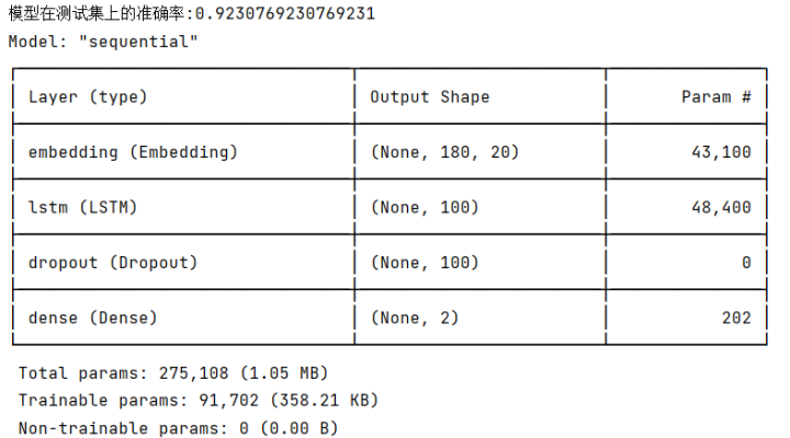
    print('模型在测试集上的准确率:%s'%acc)

    # 输出模型信息
    model.summary()
    plot_model(lstm_model, to_file='./model_lstm.png', show_shapes=True)
if __name__=='__main__':

    filepath='data/data_single.csv'
    input_shape=180
    model_save_path='data/corpus_model.h5'
    model_train(input_shape,filepath,model_save_path)    

输出结果：

Pytorch实现：

import torch
import torch.nn as nn
import torch.optim as optim
from torch.utils.data import Dataset, DataLoader
import numpy as np
import pandas as pd
import pickle
from torch.nn.utils.rnn import pad_sequence
from torchsummary import summary  # 需要安装 torchsummary

# 数据集类
class TextDataset(Dataset):
    def __init__(self, x, y):
        self.x = x
        self.y = y

    def __len__(self):
        return len(self.x)

    def __getitem__(self, idx):
        return torch.tensor(self.x[idx], dtype=torch.long), torch.tensor(self.y[idx], dtype=torch.long)

# LSTM 模型
class LSTMModel(nn.Module):
    def __init__(self, vocab_size, output_dim, n_units, label_size, dropout=0.2):
        super(LSTMModel, self).__init__()
        self.embedding = nn.Embedding(vocab_size + 1, output_dim, padding_idx=0)
        self.lstm = nn.LSTM(output_dim, n_units, batch_first=True)
        self.dropout = nn.Dropout(dropout)
        self.fc = nn.Linear(n_units, label_size)

    def forward(self, x):
        embedded = self.embedding(x)
        lstm_out, _ = self.lstm(embedded)
        out = self.dropout(lstm_out[:, -1, :])  # 取最后一个时间步的输出
        out = self.fc(out)
        return out

# 加载数据
def load_data(filepath, input_shape=20):
    df = pd.read_csv(filepath)

    # 标签及词汇表
    labels, vocabulary = list(df['label'].unique()), list(df['evaluation'].unique())

    # 构造字符级别的特征
    string = ''
    for word in vocabulary:
        string += word

    vocabulary = set(string)

    # 字典列表
    word_dictionary = {word: i + 1 for i, word in enumerate(vocabulary)}
    with open('word_dict.pk', 'wb') as f:
        pickle.dump(word_dictionary, f)
    inverse_word_dictionary = {i + 1: word for i, word in enumerate(vocabulary)}
    label_dictionary = {label: i for i, label in enumerate(labels)}
    with open('label_dict.pk', 'wb') as f:
        pickle.dump(label_dictionary, f)
    output_dictionary = {i: labels for i, labels in enumerate(labels)}

    # 词汇表大小
    vocab_size = len(word_dictionary.keys())
    # 标签类别数量
    label_size = len(label_dictionary.keys())

    # 序列填充，按input_shape填充，长度不足的按0补充
    x = [[word_dictionary[word] for word in sent] for sent in df['evaluation']]
    x = [torch.tensor(seq[:input_shape] + [0]*(input_shape - len(seq))) if len(seq) < input_shape else torch.tensor(seq[:input_shape]) for seq in x]
    y = [label_dictionary[sent] for sent in df['label']]

    return x, y, output_dictionary, vocab_size, label_size, inverse_word_dictionary

# 模型训练
def model_train(input_shape, filepath, model_save_path):
    # 加载数据
    x, y, output_dictionary, vocab_size, label_size, inverse_word_dictionary = load_data(filepath, input_shape)

    # 将数据集分为训练集和测试集，占比为9：1
    train_size = int(0.9 * len(x))
    train_x, test_x = x[:train_size], x[train_size:]
    train_y, test_y = y[:train_size], y[train_size:]

    # 创建数据加载器
    train_dataset = TextDataset(train_x, train_y)
    test_dataset = TextDataset(test_x, test_y)
    batch_size = 32
    train_loader = DataLoader(train_dataset, batch_size=batch_size, shuffle=True)
    test_loader = DataLoader(test_dataset, batch_size=batch_size, shuffle=False)

    # 模型输入参数，需要根据自己需要调整
    n_units = 100
    output_dim = 20

    # 初始化模型、损失函数和优化器
    model = LSTMModel(vocab_size, output_dim, n_units, label_size)
    criterion = nn.CrossEntropyLoss()
    optimizer = optim.Adam(model.parameters())

    # 训练模型
    epochs = 100
    for epoch in range(epochs):
        model.train()
        total_loss = 0
        for batch_x, batch_y in train_loader:
            optimizer.zero_grad()
            outputs = model(batch_x)
            loss = criterion(outputs, batch_y)
            loss.backward()
            optimizer.step()
            total_loss += loss.item()
        print(f'Epoch {epoch+1}, Loss: {total_loss / len(train_loader)}')

    # 保存模型
    torch.save(model.state_dict(), model_save_path)

    # 测试模型
    model.eval()
    correct = 0
    total = 0
    with torch.no_grad():
        for batch_x, batch_y in test_loader:
            outputs = model(batch_x)
            _, predicted = torch.max(outputs, 1)
            total += batch_y.size(0)
            correct += (predicted == batch_y).sum().item()
    print(f'Test Accuracy: {correct / total}')

    # 输出模型结构摘要
    #dummy_input = torch.randint(0, vocab_size, (1, input_shape), dtype=torch.long)
    #dummy_output = dummy_input.long()
    #summary(model, input_size=dummy_input.shape,device='cuda')

# 加载模型
def load_model(model_path, vocab_size, output_dim, n_units, label_size):
    model = LSTMModel(vocab_size, output_dim, n_units, label_size)
    model.load_state_dict(torch.load(model_path,weights_only=True))
    model.eval()
    return model

if __name__ == '__main__':
    filepath = 'data/data_single.csv'
    input_shape = 180
    model_save_path = 'data/corpus_model.pth'

    # 训练模型
    #model_train(input_shape, filepath, model_save_path)

    # 加载模型
    x, y, output_dictionary, vocab_size, label_size, inverse_word_dictionary = load_data(filepath, input_shape)
    n_units = 100
    output_dim = 20
    loaded_model = load_model(model_save_path, vocab_size, output_dim, n_units, label_size)

    # 输出模型结构摘要
    #dummy_input = torch.randint(0, vocab_size, (1, input_shape), dtype=torch.long)
    #dummy_output = dummy_input.long()
    #summary(loaded_model, input_size=dummy_input.shape, device='cuda')

    # 测试加载的模型
    #loaded_model.eval()
    correct = 0
    total = 0
    with torch.no_grad():
        for batch_x, batch_y in DataLoader(TextDataset(x, y), batch_size=32, shuffle=False):
            outputs = loaded_model(batch_x)
            _, predicted = torch.max(outputs, 1)
            total += batch_y.size(0)
            correct += (predicted == batch_y).sum().item()
    print(f'Loaded Model Accuracy: {correct / total}')

运行效果：

D:\miniconda3\envs\nlp_gpu_env\python.exe D:\AI_Course_bak\nlp_project\chapter06\LSTMDemo.py 
D:\AI_Course_bak\nlp_project\chapter06\LSTMDemo.py:21: UserWarning: To copy construct from a tensor, it is recommended to use sourceTensor.clone().detach() or sourceTensor.clone().detach().requires_grad_(True), rather than torch.tensor(sourceTensor).
  return torch.tensor(self.x[idx], dtype=torch.long), torch.tensor(self.y[idx], dtype=torch.long)
Epoch 1, Loss: 0.69065481867672
...
Epoch 100, Loss: 0.006949104128159152
Test Accuracy: 0.9347319347319347
Loaded Model Accuracy: 0.9927620826523464
Process finished with exit code 0

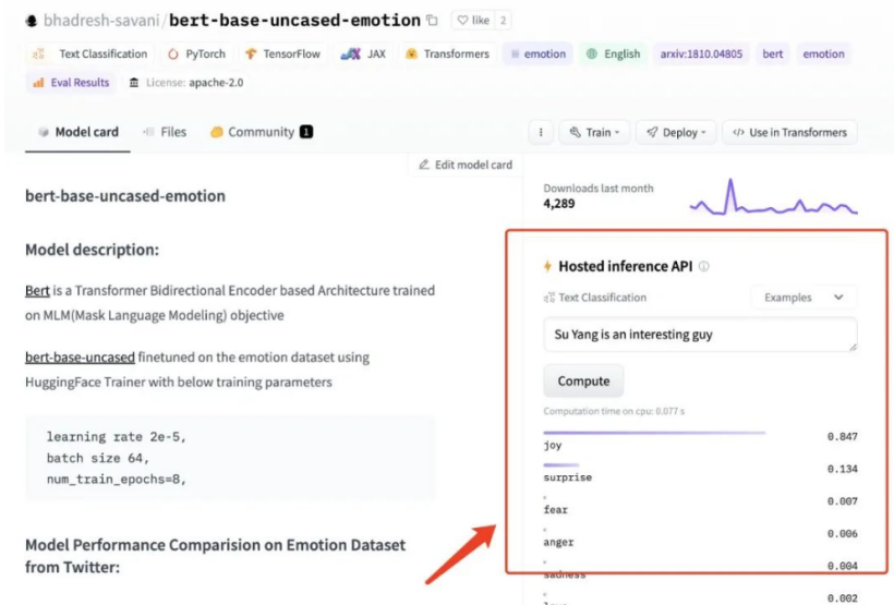
3.使用Huggingface实现基础的文本分析功能

我在 HuggingFace 上找到了一个效果还不错的预训练模型：bhadresh-savani/bert-base-uncased-emotion。它是基于“镇站之宝”，上个月下载量有三千三百万之多的 bert-base-uncased 基础上优化得出的，这个模型在英文内容的情感分析准确率能够达到 94%，看起来还是比较不错的。

下载模型：

huggingface-cli download --resume-download bhadresh-savani/bert-base-uncased-emotion --local-dir g:/ai_model/bhadresh-savani-bert-base-uncased-emotion

简单英文文本情感分析。

from transformers import pipeline
import os

os.environ['HF_ENDPOINT'] = 'https://hf-mirror.com'
classifier = pipeline("text-classification",model='bhadresh-savani-bert-base-uncased-emotion', top_k=1)
#prediction = classifier("Good Good Study, Day Day Up" )
#prediction = classifier("今天去爬山了，玩的真开心!" )
#prediction = classifier("今天数学期末考试，最后一道大题没有做出来，很是郁闷。" )
prediction = classifier("I didn't manage to solve the last big question in the math final exam today, which is quite frustrating." )
print(prediction)

运行结果：

[[{'label': 'anger', 'score': 0.6561141014099121}]]

4.实现基础的文本翻译功能

和上文中挑选情绪分析模型一样，想要实现中文翻译为英文，同样我们需要先找一个效果还不错的模型。我写了一句比较无厘头的测试内容，对这些模型进行测试：“ 张无忌抄起一张板凳，将成昆拍晕了过去。 ” 经过精心挑选，penpen/novel-zh-en 模型的翻译结果：“Zhang Wuji picked up a stool and knocked Cheng Kun unconscious.”更对我的胃口。那么就基于它来实现应用功能吧。还是先来实现基础的模型能力，“翻译”功能相关的程序。想要让模型正确运行，我们除了需要安装“情感分析”模型需要的transformers 和 torch 之外，还需要安装下面两个依赖：

pip install pip install sentencepiece sacremoses -i https://pypi.tuna.tsinghua.edu.cn/simple

还是老样子，简单写几行代码，来完成模型的调用，验证程序是否能够正常运行：

from transformers import pipeline
import os
import torch

#测试pytorch和cuda环境
print(torch.__version__)
print(torch.version.cuda)
print(torch.cuda.is_available())

os.environ['HF_ENDPOINT'] = 'https://hf-mirror.com'

translator = pipeline("translation", model="penpen-novel-zh-en", max_time=7, device='cuda')
#prediction = translator("张无忌抄起一张板凳，将成昆拍晕了过去。", )[0]["translation_text"]
#prediction = translator("不要妄下结论，‌先把事情搞清楚。", )[0]["translation_text"]
#prediction = translator("我妹妹很固执，‌你要她改变心意根本就是白费力气。", )[0]["translation_text"]
prediction = translator("我家里有些闲钱可以借给你。", )[0]["translation_text"]
print(prediction)

运行效果：

2.3.1
12.1
True
Special tokens have been added in the vocabulary, make sure the associated word embeddings are fine-tuned or trained.
I have some free money to lend to you at home.

5.使用gradio实现翻译+情感分析web应用

实现代码：

import gradio as gr
from transformers import pipeline

classifier = pipeline("text-classification", model="bhadresh-savani-bert-base-uncased-emotion", top_k=1,device='cuda')
#现在这个翻译模型仅仅实现了中文翻译为英文，其实咱们也可以下载对应的英文翻译为中文的模型。
translator = pipeline("translation", model="penpen-novel-zh-en", max_time=7,device='cuda')

def doAnalytics(input):
    return classifier(doTranslate(input))[0]

def doTranslate(text):
    translation = ""
    split_text = text.splitlines()
    for text in split_text:
        text = text.strip()
        if text:
            if len(text) < 512:
                sentence = translator(text)[0]["translation_text"] + "\n\n"
                translation += sentence
                print(split_text)
            else:
                for i in range(0, len(text), 512):
                    if i + 512 > len(text):
                        sentence = translator(text[i:])[0]["translation_text"]
                    else:
                        sentence = translator(
                            text[i: i + 512])[0]["translation_text"]
                    translation += sentence
    return translation


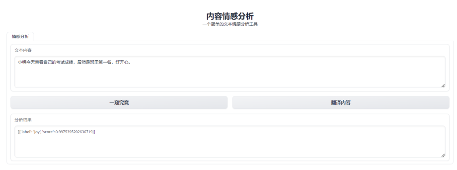
with gr.Blocks() as demo:
    gr.Markdown("<center><h1>内容情感分析</h1> 一个简单的文本情感分析工具</center>")
    with gr.Tab("情感分析"):
        with gr.Row():
            with gr.Column(scale=1, min_width=600):
                input = gr.Textbox(label="文本内容", lines=4, max_lines=100, placeholder="等待分析的文本内容...")
                with gr.Row():
                    analytics_button = gr.Button("一窥究竟")
                    translate_button = gr.Button("翻译内容")
                output = gr.Textbox(label="分析结果", lines=4, max_lines=100, placeholder="分析结果...")
    analytics_button.click(doAnalytics, api_name="analytics", inputs=[input], outputs=output)
    translate_button.click(doTranslate, api_name="translate", inputs=[input], outputs=output)

# 定义端口号
gradio_port = 8080
gradio_url = f"http://127.0.0.1:{gradio_port}"
demo.launch(
    debug=True,
    server_name="127.0.0.1",
    server_port=gradio_port
)

运行效果：